Physics of Econophysics

Yougui Wang$^1$, Jinshan Wu$^{1,2}$, Zengru Di$^1$
1. Department of System Science at School of Management,
Beijing Normal University, Beijing, 100875, P.R.China
2. Department of Physics, Simon Fraser University, Burnaby, B.C. Canada, V5A 1S6

Abstract:

Econophysics is a new area developed recently by the cooperation between economists, mathematicians and physicists. It's not a tool to predict future prices of stocks and exchange rates. It applies idea, method and models in Statistical Physics and Complexity to analyze data from economical phenomena. In this talk, three examples from three active main topics in Econophysics are presented first. Then using these examples, we analyze the role of Physics in Econophysics. Some comments and emphasis on Physics of Econophysics are included.

Introduction

Econophysics is a developing field in recent years. It's a subject applying and proposing idea, method and models in Statistical Physics and Complexity into analyzing data coming from economical phenomena. Economics is a subject about human behavior related with the management of the resources, finances, income, the production and consumption of goods and services. So Economics is usually regraded as a social science. But in some ways, the laws in Economics are similar with natural science. Although it has to deal with incentive and human decision, but sometimes the collective behavior can be described by determinant process, at least in a statistical way. So the aim of Econophysics is to apply the idea of natural science as far as well into economics. Maybe this will disentangle natural laws and human behaviors in economical phenomena, and end with a new Economics.

Also because of the plenty data records of different systems in our economy behavior, it's a treasure to physicists, especially to the one being interested in Complex Systems, in which many subsystems and many variables interact together. And the development of Economics also provide many open questions, like stock price, exchange rate and risk management, which may require technics dealing with mass data and complex systems.

Physics tries to construct a picture of the movement of the whole nature. Mechanism is the first topic cared by physicists. So trying to describe and understand the phenomena is the first step of econophysicists facing the mass data in economical phenomena. Till now, we have to say, the most works in Econophysics are empirical study of different phenomena to discover some universal or special laws, and also some initial effort about models and mechanism.

Therefor, in this talk, we will begin with three examples of empirical works in Econophysics, and discuss very shortly about the corresponding models and mechanism. Focus will be on the Physics of Econophysics, to present the power of Physics to Econophysics and some benefit which Physics will get from Econophysics.

Three main topics of Econophysics

Recent works in Econophysics mainly in three objects. First one is the time series of stock prices, exchange rates and prices of goods. Size of firms, GDP, individual wealth and income are the second topic, which can be regarded as wealth of different communities. The third one is network analysis of economical phenomena.

Fluctuation of stock prices and exchange rates

The prices of stocks are recorded every minute or every few second everyday in stock market all over the world. The price of a stock is driven by many factors, such as the whole economy environment, achievement of enterprise, the prices of other stocks, and by the buying or selling activity of stockholders. At the same time, the behavior of stockholders is effected by the price, and further more, everyone has his/her own decision which is different with each other, but effected each other. So such phenomena seem complex. While every enterprise has its own characters, and every stockholder decide his/her behavior on his/her own knowledge, information and belief, and every stock market has its own environment, the empirical study shows some common stylized facts valid for almost all stocks.

A typical time series of stock price, S$\&$P500 index, denoted as $S\left(t\right)$, is showed in figure 1. Actually S$\&$P500 is a stock index, which is a weighted mean value of stocks in a market, can be used as a indicator of stock price. Some papers use the data of indexes, some use individual stock, and also some paper investigate all stocks in a market as an ensemble of stocks. In this talk, we just use analysis of individual stock as examples.

Fig 1: Figures extracted from [5], time series of stock price. The first two figures at bottom are time series of return while the last one is a Gaussian noise

Because economy is in growth, so the time series of stock price has a long term trend to increase. This means it's nonstationary. So other than the original price, other quantities like different and return may be better to use as analysis object. The difference is defined as

$$D_{\Delta t}\left(t\right)=S\left(t+\Delta t \right)-S\left(t\right),$$ (1)

in which $\Delta t$ is the time step to sample the time series. It can be the time step of record, or a large time scale. Return is defined as

$$G_{\Delta t}\left(t\right)=\ln\left(S\left(t+\Delta t \right)\right)-\ln\left(S\left(t\right)\right).$$ (2)

It's equivalent with $\frac{D_{\Delta t}\left(t\right)}{S\left(t\right)}$ when $\Delta t$ is small enough.

Most works use return as object time series. The figures in the lower part of figure 1 show examples of $G\left(t\right)$, while the last one is a Gaussian noise signal for comparison.

A statistical analysis of one time series can be classified as two parts, the distribution properties which dismiss the time information, and the autocorrelation analysis which mainly takes time into account.

Distribution properties

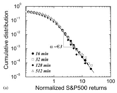
The frequency account of a data set formed by collecting all the return values will give us the distribution, as shown in figure 2.

Fig 2: Figures extracted from [5], distribution of return. Log-normal for central part and power law heavy tail.

Detailed fitting shows the central part is a log-normal distribution ( $p(x)\sim e^{-\ln^{2}x}$) while the tail is a power law distribution ( $p(x)\sim x^{-\alpha}$). The more important thing here is the universality. The distribution shape is independent on the time scale ($\Delta t$), and is a common distribution for different stocks in different markets, even in different countries. When an empirical statistical result is universal, we have to ask for the common nature behind it.

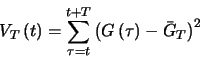
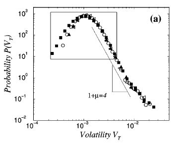
Another distribution properties is about the volatility of stock, which is related with risk. So its characters is important for risk management. Usually it's defined by local variation,

$$V_{T}\left(t\right)=\sum^{t+T}_{\tau=t}\left(G\left(\tau\right)-\bar{G}_{T}\right)^2$$ (3)

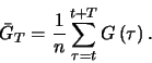
in which $T=n\Delta t$ is a time window moving along with the time, and $\bar{G}_{T}$ is the mean value of $G\left(t\right)$ in the window, as

$$\bar{G}_{T}=\frac{1}{n}\sum^{t+T}_{\tau=t}G\left(\tau\right).$$ (4)

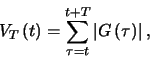
In some papers, volatility is also defined as

$$V_{T}\left(t\right)=\sum^{t+T}_{\tau=t}\left\vert G\left(\tau\right)\right\vert,$$ (5)

in which absolute value is equivalent with square, and we don't care about the mean value of $V_{T}$, which can be set to be zero when we analysis the distribution function or autocorrelation. Also it was found that the distribution function is universal for different stocks in different market during different time. Similarly the center part is log-normal, while the tail is power law, which is shown in figure 3.

Fig 3: Figures extracted from [9], distribution of volatility. Log-normal for central part and power law heavy tail.

Autocorrelation

Besides the distribution property, most information of time series is included in time. Now we present the result of autocorrelation analysis of return and volatility[5]. The autocorrelation of a stationary time series is defined as

$$C\left(\tau\right) = \frac{\langle G\left(t+\tau\right)G\l... ...^{2}\left(t\right)\rangle-\langle G\left(t\right)\rangle^{2}}$$ (6)

It can be investigated by spectrum analysis. But for a nonstationary one, a recently developed detrend fluctuation analysis (DFA)[35] is commonly used.

In figure 4, the autocorrelation functions of return and volatility are plotted together. We can find an exponential drop off in return with a time scale of minute, while a power law decrease in volatility without a finite time scale. Think about this phenomenon, a time series almost without an autocorrelation, but a extremely high autocorrelation in absolute value, or local variation. It's amazing. The fast dropping off guarantee the validness of Efficient Market Hypothesis, while the long time autocorrelation in volatility make it possible to construct a theory of risk management. So such works will boost the development of risk management, even a reformation.

Fig 4: Figures extracted from [9], autocorrelation of return and volatility. Exponential decay for return while power law decay for volatility.

Price and volume

All the analysis above looks like kinetics, which solve the question how to describe the movement and what's the movement. The next question in the tradition of Physics is how can such movement happen. So next step, let's think about what are the factors effect the stock price. And again, we may try to keep our eyes on empirical study as far as we can. Demand and supply decide the price is a central law in Economics. Although we know it's for price of goods, maybe it will still be valid for stocks. 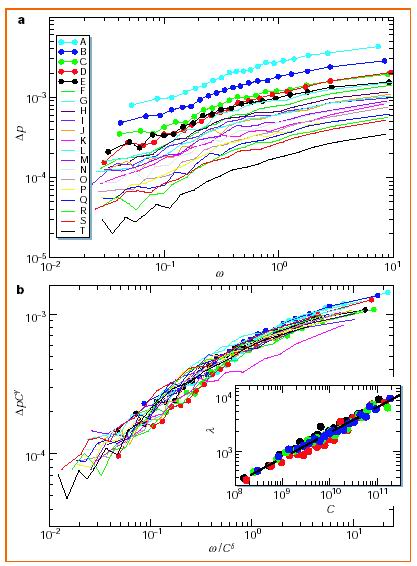So it leads us to empirical study of order book of stocks, which study the relation between difference of prices and the transaction volume[16,17]. For a individual stock, they recorded transaction volume $\omega$ as the total volume of every transaction before the price changed, and define the difference of the logarithm of the price now and price before such change as price shift,

$$\Delta p\left(t_{i+1}\right)=\ln S\left(t_{i+1}\right) - \ln S\left(t_{i}\right).$$ (7)

Then plots of price shift ( $\Delta p\left(t\right)$) vs transaction volume ( $\omega\left(t\right)$) are presented in the up part of figure 5. In the lower part, the authors found all curves can be collapse onto a common line by rescale. So it's also a universal law for all stocks.

Fig 5: Figures extracted from [16], A master curve for the relation between price and volume.

From the above results, it seems that stock price is only determined by transaction volume. But it's sad to say, the transaction volume is also decided by price. No direct way to predict transaction volume. It should be decided together with price by other predictable or known variables. So let's say if we have only one stock, and the whole history of this stock is already known, the achievement and activity of the enterprise is also predictable by other ways, and so is the external economy environment, at least in a statistical way, which means if they are random variables we know the distribution and correlation, in such condition, is the future of this stock determinant, and is it predictable or chaotic? Or at least we can reproduce the similar data with the same statistical characters as the empirical data? If it's possible, what's the central variables, and how it can be generalized into a stock ensemble, not only one stock?

Toy models

The questions above ask for a mechanism model of stocks. Maybe it's not very possible to reproduce the exact time series, but if the stylized statistical facts are reproduced, the model is well done in physical sense, although not in a sense of making money. Let's check what's the central variable left after so many things settled down by us including initial condition (even history), boundary condition (only one stock), external variables (enterprise and environment). So the only one thing left here is how do stockholders buy and sell the stock under different price and how does the price effected by the transaction.

The first idea here is activities of all stockholder are effected each other. Such interaction maybe is indirectly through the price and market, or by external way such as personal relationship. As a tradition in Physics, a first approximation is treat every stockholder independently, so they will only effected each other through market. Like in spin model, every stockholder will has a unit volume can buy or sell every time. Buying will improve the price while selling lowers the price. Everyone is trying to make more money in this game. So till now, a toy model has been constructed for mechanism of stock price. When the detail of benefit evaluation of every player and the effect on price by one unit volume is set, this toy model will evolute in its own way, of course when some specific behavior of all external variables are also settled down.

Although it's only a toy model, we also can test some fundamental knowledge, such as benefit and rational agent, and also try different form of external variables. For example, we can take for granted that external variables are random signals with fixed distribution and without autocorrelation of any order. So our task will be how can we construct our model to reproduce the autocorrelation behavior in empirical study from no autocorrelation input external data.

And then, if the output data is totally incomparable, maybe we have to add something we dismissed, like the relation between stocks. You know a phone call from your close friend may change your decision. So it's very possible we have to take such interaction into consideration. The model in [10], is a representative one of such toy models. Although many different interaction forms we can try, or even we can coevolute the interaction strength together with the stock price, it's possible that the output data is still incomparable with empirical one. Then, we will have to include the interaction between different stocks, and maybe further more a coevolution system including the behavior of enterprises.

Oh, no, wait a minute, this is not on the way of physics now. More and more variables, more and more subsystems, uglier and uglier picture. It shouldn't. The Physics of Complex System tells us maybe only a few ones rule the system. So the toy model maybe imply something valuable. Now we come back to empirical study and toy model, but in another way, the way keeping Physics in mind.

Goods, options and others

Not only the stocks, also exchange rates, goods and options are under analysis nowadays. However, the universal results for stocks seems not valid for other goods and options. The empirical study of land price[31] gives the high skew and heavy tail distribution of price ( $S\left(t\right)$) and power law distribution for relative price ( $r\left(t\right)=\frac{S\left(t+1\right)}{S\left(t\right)}$. And empirical study of return of options shows unsymmetrical power law distribution[33]. And not only the prices, waiting time can also be take into consideration. In a real stock market, transactions do not always happen in every minute or every half minute. It's also a random variable. And the prices change depending on the transactions. This is the so-called continuant time stochastic process. Empirical and model analysis just started up[11,12,13].

Distribution of firm sizes, GDP, personal income and wealth

Interaction between different communities such as trade, cooperation and competition, plays important roles in economy. As a result of such activities, the wealth distribution carries some valuable information for researchers to investigate the properties of such interaction. So the second active main topic in Econophysics is about the size distribution. For a firm, size can be measured by employee, sales or capitals, while GDP for a country, income or wealth for a person.

Distribution of size

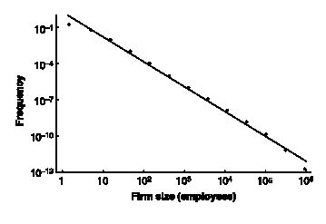
In [22], the author collected data including more firms especially small firms in a longer history than the database in [21], so the result of power law distribution seems more convincing than the log-normal distribution in the later. And the important character about such distribution is the universality. Different measurement of size such as total employees, sales, assets and capitals give the same distribution. And it doesn't depend on the time, even during the years of significant change of working force. Further investigation[24] shows it's also a common law in different countries. A typical distribution is shown in figure 6.

Fig 6: Figures extracted from [22] and [27], Zipf plot of sizes of firm, and Zipf plot of size of GDP of countries, nearly a perfect power law.

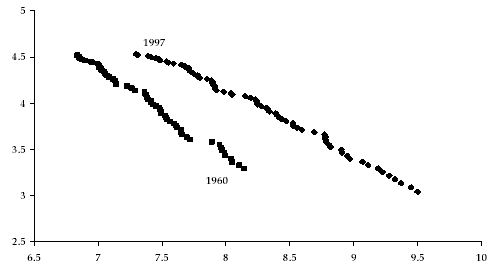
Similar results have been get for GDP of countries all over the world. Power law distribution of GDP per capita of different counties has been revealed in [27].

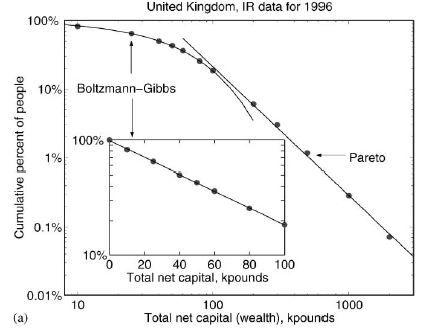
For individual such distribution can be analyzed by personal income or wealth. A typical result[29,30] is shown in figure 7. The lower income seems like exponential distribution while the higher part is power law. From experience of ideal gas, we know, the equilibrium energy distribution of a random exchange system is exponential. So maybe in the lower income community, the cooperation and competition between individuals is in a way similar with random exchange. But for the higher income part, different interaction like preferential attachment part more important role.

Fig 7: Figures extracted from [29], Cumulative Distribution Function of individual income and wealth.

Growth rate

Growth rate of firm size is defined similarly with return as

$$r\left(t\right)=ln\left(S\left(t+1\right)/S\left(t\right)\right).$$ (8)

Then in an ensemble of firms, every firm has its own track, and at every time, we have a cross-section data set including all firms. In a tradition of Statistical Physics, analysis can be done along two ways, keeping eyes on individual time series or just dealing with cross-section data. In an ensemble consist of identical systems, those two ways will give the same result. However, although here we can make an assumption that all firms act in a common way, which is the way we want to find, our ensemble is not consist of identical systems. So the compromise here was to treat the firms with the same size as identical systems, and to dismiss the time information and mix them together. 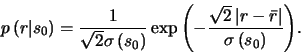At last, we will have conditional distribution function for different size as $p\left(r\vert s_{0}\right)$, where $s_{0}$ is the initial form size. Actually, such analysis is on the first way we mentioned, keeping eyes on fixed firm, so we get $p\left(r\vert s_{i0}\right)$, where $i$ is the label of firm. 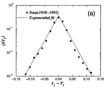But here, a little further we go, the tracks starting at the same size are combined together. The distribution of growth rate is shown in figure 8 as Laplace distribution,

Fig 8: Figures extracted from [26] and [28], Distribution of growth rate of GDP.

$$p\left(r\vert s_{0}\right)=\frac{1}{\sqrt{2}\sigma\left(s_{... ...vert r-\bar{r}\right\vert}{\sigma\left(s_{0}\right)}\right)}.$$ (9)

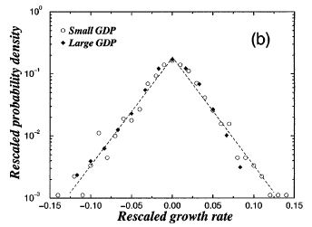
Similar growth rate analysis has also been done for GDP. The gross growth rate of GDP is defined as

$$p_{i}\left(t\right)=\ln\left(\frac{G_{i}\left(t+1\right)}{G_{t}\left(t\right)}\right).$$ (10)

But since the long term growth trend of economy, when we want to analysis the fluctuation information, such endogenous unknown trend has to been excluded. In [28], the author suggested to use a decomposition as below,

$$p_{i}\left(t\right) = \delta_{i} + \phi\left(t\right) + r_{i}\left(t\right),$$ (11)

where $\delta_{i}$ is the long term expected endogenous growth rate, $\phi\left(t\right)$ is a common fluctuation to all counties, and $r_{i}\left(t\right)$ is the residual which represents fluctuation, the one we want to investigate. As shown in Fig 8-(b), it has the same Laplace distribution.

Relation between fluctuation and size

From experience in Statistical Physics, relation between fluctuation and size usually gives important information of the underlying processes[26]. Like in idea gas with independent particles, the magnitude of fluctuation is invert of the square root of the system size as

$$\sigma\left(N\right)\sim N^{-\frac{1}{2}}.$$ (12)

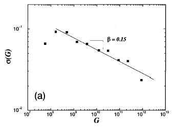
Corresponding analysis can be done for growth rate of firm size and GDP. A power law relation but with exponent other than $-\frac{1}{2}$ has been revealed by researchers[26,28], as shown in figure 10. And further more, such exponents is universal for different measurement of firm size, independent on time and locations, and the values for firm size and GDP is very close. So maybe this implies some common mechanism for firms and GDPs.

Fig 8: Figures extracted from [26] and [28], Relation between variation and size.

Complex Networks of economy systems

Economy is a many-body system including agents as individuals, firms, countries, goods as produce, production and service, and subsystems as financial system, manufacturing, agriculture, service industry. And all of them interact with each other. A general way developed recently to describe such system is Complex Networks. In a complex network, every agent is represented by a vertex and the interaction between any two agents is described by a link between the two corresponding vertexes. Further more, the weight of links can be used as the strength of the interaction and a directed link can be used when the interaction is not symmetrical.

A recent such development is the web of trade[14,15], in which vertexes are the countries and links are the inport/outport relation. The basic structure and efficiency has been analyzed, like high clustering coefficient, scale-free degree distribution.

Another widely used network of economy system is the interaction between stock agents. Every stockholder is a vertex in the network, and the effect from decision of one agent to another is a directed link from the former vertex to the later. So the network acts as a whole system to drive the stock price. The geometrical character of such network will have some important effects on the dynamical behavior of stock price. Therefor, such investigation maybe will reveal the interaction pattern between stock agents.

The third proposed works about network of economy systems is the network analysis of product input/output table. Like the Predator-Prey Relationships in food web, every product made from other products or raw materials, and also become input of other products. So the input/output relationship between products forms a network. Actually the input/output table analysis in Economics has the same spirit but in a highly clustered level and asking for different questions. So, although a database of product relation is what we need, a clustered group product relation data set will also be able to be used here as an beginning analysis of basic structure characters. And further works will require detailed data on input/output relation of products.

Construction and analysis of such clustered product network is in progress[36]. Characters on degree distribution, clustering coefficient, weight and weight distribution, average shortest distance have been gotten, but questions about the universality of such properties need to be tested on more networks. The links between products can be regarded as technology. So a score analysis such as link betweenness will show the relative importance of different technics, therefor it may imply some new direction of development of technology. Further questions about the robustness of such networks can be asked as how many total product will be lost if one or several inter-products were in shortage, or when the resource distribution was changed, or as how many total product will be lost when one or several link (technics) were dismissed, or inversely, if a new link was invented how many product will grow in total. Such investigation will relate traditional questions in economics such as resource allocation, social welfare, and effect of new technology with network analysis of product. It can have a far-reaching effect both on economics and network analysis.

Why is Econophysics?

We took a review of Econophysics including empirical study and models on three topics above. Now we try to discuss the question why is Econophysics? Since dynamics of Stock price is also a topic of Mathematical financial, what's the difference between this and Econophysics? If Physics provide insightful tools for this new field, can Physics also benefit from it?

Physics as tools

First, let's discuss the role of Physics as tools in Econophysics, the application of concepts, models and method developed in Physics into Econophysics.

Physics as analysis method

There is many-years experience to deal with many-body system and complex system in Physics. The concepts and technics such as ensemble statistics, correlation and self-correlation analysis, have been widely used to reveal the property of economy phenomena. And the more important thing here is experience in Physics helps to understand what the properties imply. For instance, a power law is usually related with critical phenomena in Physics, including critical point of equilibrium and non-equilibrium phase transition. And so does a long range order and a high self-correlation. Also as pointed in [26], relation between variation and size imply the form of interaction.

Another central analysis method transplanted from Physics is Data Collapse and Universality. If relation curves from different systems can be collapsed onto a master curve by scaling, it's very possible to find some common mechanism from such systems. And if an empirical or theoretical relation is independent on time period, some different detail of objects, it's called universality. When a universal law is found for different systems, the systems must be equivalent in some ways. So it implies common mechanism and others can be understood if we know one of them very well. Therefor, it open a new way to investigate such systems, especially when some models with similar properties in Physics and other fields can be used here as a reference model for economy phenomena.

Physics as reference model

Spin model is widely used to describe human decision in stock market[] or other economy activity[]. Usually, status of an agent can be one of $\left\{1,0,-1\right\}$, which is interpreted as buying, waiting and selling, or one of $\left\{1,-1\right\}$. So the status space of the whole system with $N$ agents is $\left(S_{1},S_{2},S_{3},\cdots,S_{N}\right)$. The benefit of every agent is determined by a payoff function $E\left(\vec{S},\vec{J},IEs\right)$, in which $\vec{J}$ are the interaction constants of all orders and $IEs$ are the internal variables as stock price, or external information like environment and behavior of enterprise. Everyone intend to maximize its own benefit in a statistical way[,] like

$$\omega_{i}\left(S_{i}\left(t\right)\rightarrow S_{i}\left(t+1\right)\right)\sim e^{\frac{\Delta E_{i}}{T}},$$ (13)

in which $T$ is an average evaluation coefficient, which means the effect on ones decision for a unit benefit. Actually such form of human decision comes from the ensemble distribution in Statistical Mechanics. In metropolis simulation of a spin system, the probability for a spin to transfer its status is overruled by a similar form. An ensemble distribution here means in statistical way, in a many body system, although everyone try to stay on maximum position, but the end status is much like an ensemble distribution.

Such application gives some reasonable results, although it may be not totally equivalent with assumption in Economics, where every agent must stay on its maximum point, not a distribution function. In Mechanics, the status of physical object is determined by Newton's equations or minimum action principle, but for a many-body system in Statistical Mechanics, ensemble distribution is used instead. Although it's not deduced from first principle, it works widely. Maybe similar approach can be developed in Economics.

Ideal gas is another reference model widely used in Econophysics[]. In a first order approximation model of competition and cooperation between firms, or between individuals, every agent can be regarded as random exchange wealth with each other, like random exchange energy in ideal gas. So the equilibrium distribution will take the exponential form. It's amazing that the central part of personal wealth is actually exponential form. Further possible model can be generalized random interaction model, including not random exchange, but also random increase or decrease process, or extended model with bias exchange model, like preferential exchange, in which rich one has higher probability to get richer.

Economics as Physics

In above section, we discussed the role of Physics in Econophysics. In this section, we ask for the inverse question, what Physics can benefit from Econophysics, not only as an insightful tool.

Economy systems as physical objects

Frankly, physicists are kinda aggressive, so is Physics. When a question asking for reason of a phenomenon in a common sense, or in a fundamental way, according to physicists it's a physical question. Econophysics is such an example. It choose the special phenomena from Economics, and ask for the reason, or mechanism in physical language. Most phenomena concerned in Econophysics exhibit universality independent on time period, detail of systems, and even different economical structure of countries. So such question is likely very much to ask the behavior of a system with known interactions, or the interaction form of a system with known behaviors. It's a typical physical question.

Like DFA method proposed by researchers in Statistical Physics from works in DNA sequence and physiologic signals, new technics can also be invented from Econophysics. Hopefully, not only technics, but also concepts and fundamental approach may also be proposed.

For instance, effect of geometrical property such as dimension and curvature on dynamical behavior is an important question in Physics. Actually it's widely studied in Physics including Relativity, Quantum Physics and especially Phase Transition and Critical Phenomena. So if geometrical quantities can be defined in Complex System, and the effect on dynamical process is known, it will partially predictable just through grasping the geometrical properties of such systems. For example, in principle, the make-from relationship between all products is tractable. So the network can be explicitly constructed, and even part of the history is known, like the things changed when reformation of technics happened. So Economics provide some nearly perfect treasure for Physics. And further more, the special character of such network will definitely require new quantities or technics to describe the effect. This will maybe boost the development of Physics.

Natural parts of human behavior

Not all human behaviors are rational or determinant, like impulsion and inspiration, but some of them, are determined by environment at least in a statistical way. Personal character affects human decision. But if all other factors could be determined by physical way like a dynamical equation, and the statistical properties of personal characters of the system were known, it will be easy to predict the behavior of the system. So the most valuable question left here is that whether we can describe economy system and human behavior by physical way as far as possible and leave something unknowable in physical sense. If it's possible, how to do it. I think, Econophysics is a good try in such sense.

Economics is a science of human behavior, but it's fortunate that Economics is not totally a science of human creativity and inspiration like fine art. This means that some part, even most part according mathematicians working in Economics, of Economics can be modelled in an abstract or mathematical form. It's interesting to point out that it's Physics the most famous masterpiece applying Mathematics into nature, not any other field of Applied Mathematics. So it's natural to incorporate Physics into Economics like to imitate masterpieces.

And through such exploration, it's possible that Physics will be widely used in social science. This will greatly extend the scope of Physics, and maybe will help Physics to deal with some hard topic such as turbulence, or more general complex systems.

Conclusion - Is Econophysics a subject of Physics?

At lease, Econophysics provides, invents and develops tools for analysis of Economy phenomena, and investigation of economy system generalizes the scope of Physics. But will Econophysics effect concepts and thought in Physics? It depends on the future. However, we are sure that both Economics and Physics can benefit from such exploration. Therefor, as a researcher in physics in the new century, or a potential economist, should we learn from each other?

Acknowledgement

Thanks is given to Fukang Fang and Zhanru Yang for their simulating discussion. And we own graduate students 2002 in System Science Department for their warm discussion and good questions. The author Wu want to give thanks to Qian Feng for her encouragement and understanding. This work is partial supported by National Natural Science Foundation of China under the Grant No. 70371072 and No. 70371073.

Bibliography

1

R. N. Mantegna and H. E. Stanley, An Introduction to Econophysics: Correlations and Complexity in Finance (Cambridge University Press, Cambridge, England, 1999).

2

J.-P. Bouchaud and M. Potters, Theory of Financial Risk (Cambridge University Press, Cambridge, England, 1999).

3

R. Cont, Empirical properties of asset returns: stylized facts and statistical issues, Quantitive Finance, 1, 223-236(2001).

4

H.E. Stanley, P. Gopikrishnan, V. Plerou, L.A.N. Amaral, Quantifying uctuations in economic systems by adapting methods of statistical physics, Physica A 287, 339-361(2000).

5

P. Gopikrishman, V. Plerou, Y.liu, L.A.N. Amaral, X. Gabaix and H.E. Stanley, Scaling and correlation in financial time series, Physica A 287, 362-373(2000)

6

V. Plerou, P. Gopikrishman, L.A.N. Amaral, M. Meyer and H.E. Stanley, Scaling of the distribution of financial market indices, Phys. Rev. E 60, 5305-5316(1999).

7

V. Plerou, P. Gopikrishman, L.A.N. Amaral, M. Meyer and H.E. Stanley, Scaling of the price fluctuations of the individual companies, Phys. Rev. E 60, 6519-6529(1999).

8

Rogério L. Costa, G.L. Vasconcelos, Long-range correlations and nonstationarity in the Brazilian stock market, Physica A 329, 231-248(2003).

9

Y. Liu, P. Gopikrishman, P. Cizeau, M. Meyer, C. Peng and H.E. Stanley, Statistical properties of the volatility of price fluctuations, Phys. Rev. E 60, 1390-1400(1999).

10

A. Krawiecki, J.A. Holyst and D. Helbing, Volatility clustering and scaling for financial time series due to attactor bublling, Phys. Rev. Lett. 89, 158701 (2002).

11

M. Raberto, R. Gorenflo, F. Mainardi, E. Scalas, Scaling of the waiting-time distribution in tick-by-tick financial data (Poster presented during the international workshop Economics Dynamics from the Physics Point of View held in Bad Honnef (Germany) on March 2000).

12

L. Sabatelli, S. Keating, J. Dudley, and P. Richmond, Waiting time distributions in financial markets, Eur. Phys. J. B 27, 273-275(2002).

13

E. Scalas, R. Gorenflo, F. Mainardi, Fractional calculus and continuous-time finance, Physica A 284, 376-384 (2000).

14

M. A. Serrano and M. Boguna, Topology of the world trade web, Phys. Rev. E 68,015101(2003).

15

X. Li, Y.Y. Jin, and G. Chen, Complexity and synchronization of the World trade Web, Physica A 328, 287-296(2003).

16

F. Lillo, J.D. Farmer and R.N. Mantagna, Master curve for price-impact function, Nature 421, 129-130(2003).

17

V. Plerou, P. Gopikrishman and H.E.Stanley, Quantify stock-price response to demand fluctuations, Phys. Rev. E 66, 027104(2002).

18

F. Lillo and R. N. Mantegna, Ensemble properties ofsecurities traded in the NASDAQ market, Physica A 299, 161-167(2001).

19

F. Lillo and R.N. Mantagna, Variety and volatility in financial markets, Phys. Rev. E 62, 6126-6134(2000).

20

J.R. Iglesias, S. Goncalves, S. Pianegonda, J.L. Vega and G. Abramson, Wealth redistributioninour small world, Physica A 327, 12-17 (2003).

21

M. Stanley, S. Buldyrev, S. Havlin, R. Mantegna, M. Salinger, H.E. Stanley, Zipf Plot and the Size Distribution of Firms. Economics Letters 49, 453-457.

22

R.L. Axtell, Zpif distribution of U.S. firm sizes, Sience, 293, 1818-1820(2001).

23

L.A.N. Amaral, S.V. Buldyrev, H. Leschhorn, P. Maass, M. A. Salinger, H.E. Stanley and M.H.R. Stanley, Scaling bahavior in Economics: I. empirical results for company, J. Phys. I France 7, 621-633(1997).

24

J.J. Ramsden and Gy. Kiss-Haypál, Company size distribution in different countries, Physica A 277, 220-227(2000).

25

L.A.N. Amaral, S.V. Buldyrev, S. Havlin, M.A. Salinger and H.E. Stanley, Power law scaling for a system interacting units with complex internal structure, Phys. Rev. Lett 80, 1385-1388(1998).

26

Y. Lee, L.A.N. Amaral, D. Canning, M. Meyer, and H.E. Stanley, Universal Features in the Growth Dynamics of Complex Organizations, Phys. Rev. Lett. 81, 3275(1998).

27

Di Guilmi, Corrado, Edoardo Gaffeo, and Mauro Gallegati, Power Law Scaling in the World Income Distribution, Economics Bulletin, Vol. 15, No. 6 pp. 1-7(2003).

28

D. Canning , L.A.N. Amaral , Y. Lee , M. Meyer , H.E. Stanley, Scaling the volatility of GDP growth rates, Economics Letters 60, 335-341(1998).

29

A.A. Dragulescu and V.M. Yahovenko, Exponential and power-law probability distributions of wealth and income in the United Kingdom and The Unite States, Physica A 299, 213-221(2001).

30

A.A. Dragulescu and V.M. Yahovenko, Evidence for the exponential distribution of income in the USA, Eur. Phys. J. B 20, 585-589(2001).

31

Taisei Kaizoji, Scaling behavior in land markets, Physica A 326, 256-264(2003).

32

A.A. Dragulescu and V.M. Yahovenko, Statistical mechanics of money, Eur. Phys. J. B 17, 723-729(2000).

33

J.L. McCauley and G.H. Gunaratne, An empirical model of volatility of returns and option pricing, Physica A 329, 178-198(2003).

34

G. Bonanno, G. Caldarelli, F. Lillo, and R.N. Mantegna,Topology of correlation based minimal spanning trees in real and model markets, arXiv:cond-mat/0211546 (2002).

35

Peng C-K, Buldyrev SV, Havlin S, Simons M, Stanley HE, Goldberger AL. Mosaic organization of DNA nucleotides. Phys Rev E 1994;49:1685-1689.

36

Klaus, Jinshan Wu, Zengru Di, and Jiawei Chen, Network analysis of physical input and output tables, in prepairation.

About this document ...

Physics of Econophysics

This document was generated using the LaTeX2HTML translator Version 2002 (1.62)

Copyright © 1993, 1994, 1995, 1996, Nikos Drakos, Computer Based Learning Unit, University of Leeds.
Copyright © 1997, 1998, 1999, Ross Moore, Mathematics Department, Macquarie University, Sydney.

The command line arguments were:
latex2html Review

The translation was initiated by Jinshan Wu on 2004-01-01